Why digital PCR Cluster Predictor?

Digital polymerase chain reaction (dPCR) is a PCR-based technology that enables the sensitive quantification of nucleic acids. In a dPCR experiment, nucleic acids are randomly distributed and end-point amplified in several thousands of partitions that act as micro PCR reactors. The partitioning process and the end-point detection of targets are the foundation of dPCR high sensitivity: each partition receives either zero or few nucleic acid copies, increasing the amplification efficiency; the end-point reaction ensures the amplification of targets to a detectable level. The signal emitted by hydrolysis probes or intercalating binding dyes is used to detect the partitions containing the targets sequence. The maximum number of fluorescence signals read in a single sample represents the major limitation of dPCR technology: the majority of dPCR system on the market is able to detect up to two fluorescence signals, limiting the experiment plexity. Several strategies were developed to overcome that limitation (Whale et al., 2016), however data analysis of multiplex assays and clustering of data generated from low input specimens are still an issue: manual annotation is time-consuming, user-dependent and has poor reproducibility.

Digital PCR Cluster Predictor (dPCP) was developed to automate the analysis of multiplex digital PCR data with up to four targets. dPCP supports the analysis multiple digital PCR systems, is independent of multiplexing geometry, and is not influenced by the amount of input nucleic acid.

How to start the analysis?

dPCP requires two types of input files:

• A file containing the raw data for each sample and reference (“.eds” for QuantStudio 3D Digital PCR System, “.csv” for QX100/QX200 Droplet Digital PCR System and other digital PCR systems). The raw data of QX100/QX200 system can be exported from QuantSoft software selecting Export Amplitude and Cluster data in the Options pane, it is fundamental to keep the default file name and prepare the plate setup always for two targets (Channel1 and Channel2), even for singleplex assays. For other digital PCR systems, the raw data have to be prepared in the same format of QX100/QX200 system:
  • upload for each sample a “.csv” file with two columns (column 1: fluorescence channel to be shown on y axis of plots; column 2: fluorescence channel to be shown on x axis of plots).
  • the file name has be structured as follow: WellID_Amplitude.csv. If it is needed to analyse the files of different experiments, ensure that the same well ID is not used multiple times as the software cannot discriminate file names with the same well ID.
• A sample table. The sample table is a csv file containing the information about the samples and the experiment settings.

Some examples of input files can be found here.

The sample table has nine columns:

1. Sample name. The name to be assigned to a sample. The samples with the same name are considerate replicates. The field is not mandatory; the samples without a name are not replicates.
2. Chip ID/Well ID. This field is mandatory. For QuantStudio 3D Digital PCR System the chip ID is required, while for QX100/QX200 Droplet Digital PCR System and other systems the well ID has to be provided (e.g. A01). Chip and well ID are used to identify the raw data files, therefore the default file name of QuantStudio 3D Digital PCR System and QX100/QX200 Droplet Digital PCR System must not be changed.
3. No of targets. This field is mandatory and must be an integer number between 0 and 4.
4. FAM target. The name of the target detected with a FAM probe.
5. Target 3. The name of the third target. If the assay has an orthogonal geometry, this field should be filled in with the name of the second target detected with a FAM probe;
6. Target 4. The name of the fourth target. If the assay has an orthogonal geometry, this field should be filled in with the name of the second target detected with a VIC/HEX probe;
7. VIC/HEX target. The name of the target detected with a VIC/HEX probe.
8. Reference. This field is optional, a reference must be provided only when sensitive analyses are needed (few positive partition for one or more targets) and/or rain is expected in sample data. For QuantStudio 3D Digital PCR System the chip ID of the reference is required, while for QX100/QX200 Droplet Digital PCR System and other systems the complete file name (with file extension) of the reference raw data file has to be provided (e.g. example_ref_Amplitude.csv). If the field is empty, the corresponding sample is used as reference to identify the empty partitions and single-target clusters with DBSCAN. In this scenario, the sample must have all the requirements to be used as reference (see below). The samples from other runs can be used as reference but in case of experiments with QX100/QX200 Droplet Digital PCR System or other systems, the name of the reference file has to be changed to remove the well ID, which could interfere with the samples well IDs. Although it is not always required for the analysis, we strongly recommend the use of reference to have faster and more accurate cluster analyses.
9. Dilution. This field is mandatory and must be a numeric value representing the dilution ratio of the sample (e.g. 1:5 dilution has to be indicated as 0.2).

The sample table has to be filled out by the user with the required information. The table format is fundamental for the analysis and must not be changed. A template can be downloaded from the Input Data panel.

The input parameters to be provided are:

• ε: input parameter for the DBSCAN analysis of the reference (See below). It represents the maximum distance between the elements within a cluster. If one value is provided, it will be applied to all reference samples. If different values have to be applied to various reference samples, the values (separated by a comma) for each reference have to be provided;
• minPts: input parameter for the DBSCAN analysis of the reference (See below). It represents the number of minimum elements to assemble a cluster. If one value is provided, it will be applied to all reference samples. If different values have to be applied to various reference samples, the values (separated by a comma) for each reference have to be provided.
• Reference quality (only for QuantStudio 3D digital PCR): an integer number between 0 and 1. It represents the quality threshold to subset the reference data. If one value is provided, it will be applied to all reference samples. If different values have to be applied to various reference samples, the values (separated by a comma) for each reference have to be provided.
• Sample quality (only for QuantStudio 3D digital PCR): an integer number between 0 and 1. It represents the quality threshold to subset the sample data. If one value is provided, it will be applied to all samples. If different values have to be applied to various samples, the values (separated by a comma) for each reference have to be provided.
• Partition volume (only for Other digital PCR systems): a numeric value indicating the partion volume in microliters spcific to the digital PCR system.
• Rain: whether the rain analysis has to be carried out.
• QC reference: whether the fraction of rain elements in the reference has to be calculated. Warning messages are displayed when the percentage of rain is high.
• Color blind plots: whether the plots have to be displayed with a palette optimized for color blindness.

The analysis can be saved as a dPCP file by clicking the appropriate button in the Results panel. The dPCP file can be uploaded in the Input Data panel to visualize and modify the analysis.

How dPCP carries-out the clustering?

The first step carried out by dPCP is the collection of data and information from the input files. When a reference is used, it is fundamental to have high-quality data as dPCP starts the identification of clusters from the reference. Once a good reference has been identified, it can be used for the analysis of all samples amplified with the same experimental conditions (e.g. same assay, primers and probes concentration, cycling protocol).
The ideal reference has:

• The same experimental settings and conditions of the corresponding sample
• Sufficient input amount to promote the formation at least of high-density empty partitions and single-target clusters;
• Negligible presence of rain;
• Non-cross-reactive probes.

dPCP identifies the empty partitions and single-target clusters in the reference using the non-parametric algorithm called density-based spatial clustering of applications with noise (Ester et al., 1996) (DBSCAN). Maximum distance (ε) between cluster elements and the number of minimum elements (minPts) to assemble a cluster are the input parameters to be chosen by the users. The Test Reference panel helps the user to identify the most suitable ε and minPts values. The usage of a reference is not mandatory: the empty partitions and single-target clusters can be directly identified in the sample. However, when the input amount is low only a few data elements are positive for each target and the DBSCAN analysis could fail in the detection of those clusters. In such a case the usage of a reference sample is fundamental for the correct clustering of the sample data.

After the identification of empty partitions and single-target clusters, their centroid position is identified by computing the arithmetic mean of the coordinates of their data elements. The distance between a cluster centroid and the centroid of empty partitions can be represented by a Euclidean vector. As the coordinates of the centroids of multi-target clusters are predicted to be the sum of the coordinates of the centroids of single-target clusters, the position of the centroid of multi-target clusters can be calculated by computing the vector sum of vectors representing the distance of the centroid the single-target clusters to the centroids of empty partitions.

The clustering analysis of sample data is carried out by the c-means algorithm (Bezdek, 1981; Lai Chung and Lee, 1994; Pal et al., 1996). The principle of fuzzy c-means algorithm is to minimize the variance within the cluster. The intra-cluster variance is defined as the sum of the squared distance of all cluster elements from the cluster centroid. The fluorescence values of sample elements and the coordinates of all centroids are used as input parameter for the analysis. The output of the c-means analysis is a matrix showing the probability of membership of the data elements to each cluster. Each data element is assigned to the cluster whose probability is the highest. If the highest probability is lower than 0.5 a data element is classified as rain and its membership is recalculated with Mahalanobis distance (Mahalanobis, 1936). Mahalanobis distance computes the distance between a point and a distribution, it is based on measuring at multidimensional level how many standard deviations away is a point from the mean of a distribution. The rain-tagged elements are assigned to the cluster with the lowest Mahalanobis distance.

Finally, the copies per partition of each target are calculated according to a Poisson model. (Hindson et al., 2011). Precision is calculated as previously described (Majumdar et al., 2015). Replicates can be combined and the copies per partition are re-calculated.

How to check the clustering results and the quality of the analysis?

The results of the dPCP analysis can be visualized in 2 panels:

• the Plots panel shows the plot of the clustering of each sample. Moreover, the user can manually change the membership of data elements. After each manual annotation, the software recalculates the concentration of the targets, showing the updated quantification in the table displayed in the same panel. The plot can be exported as an image, choosing the file format and dpi.
• the Results panel shows two tables with the quantification of the targets. The upper table displays the results by replicate whereas the second table reports the results by sample. The tables can be exported to csv files. The user can also export a pdf report displaying the plot, the input settings, and the targets quantification of each sample.

Quality controls were developed to have a graphical view of the results and to check the quality of the fundamental steps of dPCP analysis. The Quality control panel shows for each sample the plot of the clusters centroid, the plot of c-means clustering and the plot of rain analysis (the latter only if the command of rain analysis is enabled in the Input Data panel). The 3 plots can be downloaded as a unique image, choosing the file format and dpi. In order to evaluate the structure of the original dPCP clustering in terms of cluster cohesion and separation, the silhouette coefficient (Rousseeuw, 1987) is displayed for each sample. According to Kaufman and Rousseeuw (Kaufman and Rousseeuw, 1990), the mean value of silhouette coefficient has to be interpreted as follow:

• between 0.71 and 1: the clustering structure is strong
• between 0.51 and 0.70: the clustering structure is reasonable;
• between 0.26 and 0.50: the clustering structure is weak and could be artificial;
• lower than 0.25: no substantial structure.

The Figure 1 shows how to interpret the quality control plot of the clusters centroid.

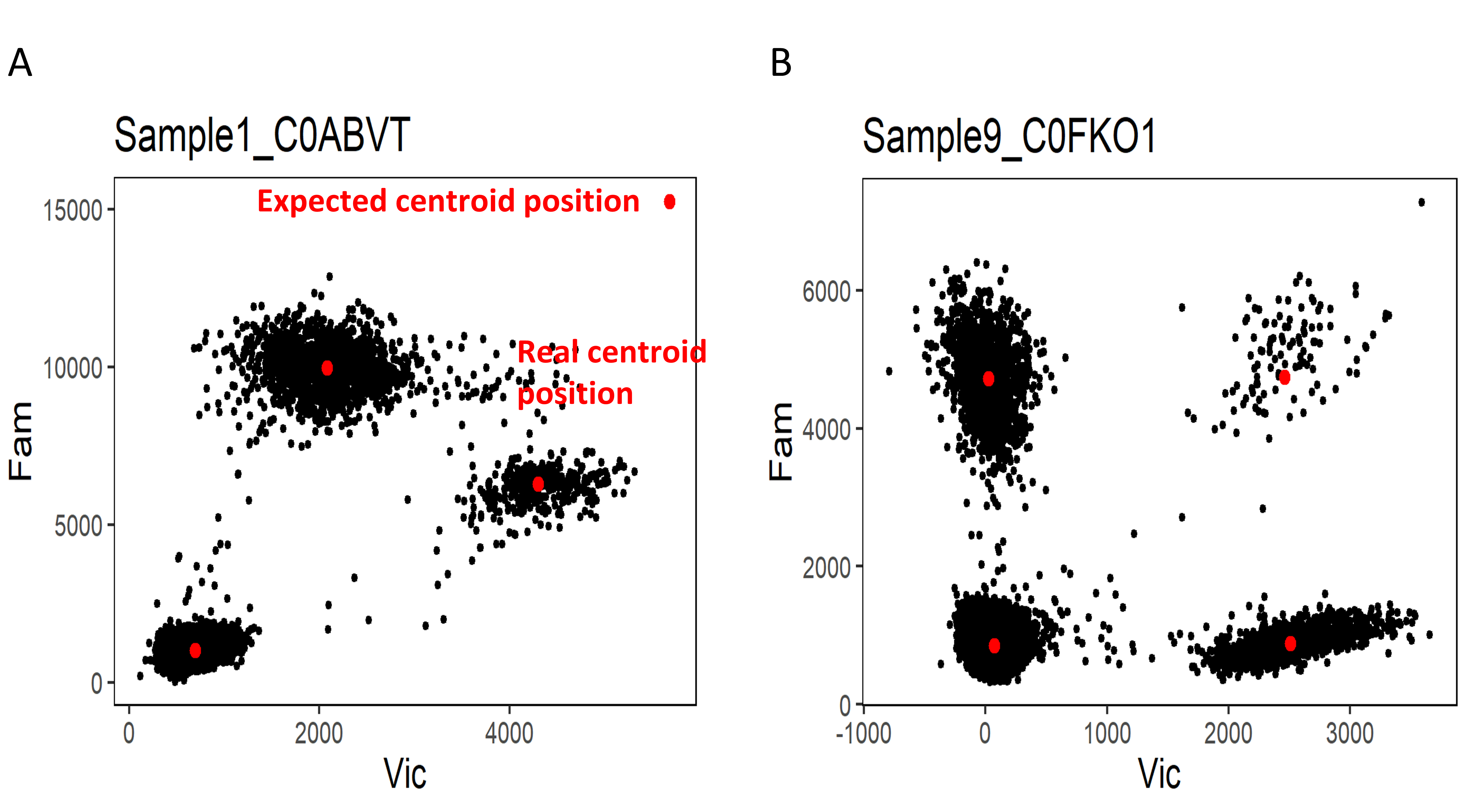
Fig. 1: Quality control of the centroids coordinates prediction. (A) The prediction of coordinates of multi-target cluster centroid did not match the real position. The shift of centroid position can be the consequence of cross-reactive probes or poor assay optimization. (B) The position of clusters centroids were correctly predicted.

In the bottom part of the Quality Control panel, the plot of the DBSCAN analysis is shown for each reference. The plot can be exported as an image, choosing the file format and dpi. The results of the DBSCAN analysis can be exported to rds file to be used as a reference in other dPCP analysis. When a rds file is used as reference, the dPCP does not need to perform a DBSCAN analysis because it retrieves the information directly from the rds file, speeding up the workflow.

Test reference

The identification of the empty partitions and single-target clusters in the reference is the first step of dPCP analysis and it relies on the DBSCAN algorithm. The performance of DBSCAN depends on the input parameters ε and minPts that are the only two values the user has to adapt for dPCP analysis. The Test Reference panel helps to choose the best input values and to select a suitable reference sample. The user has to upload the raw data file (see How to start the analysis?) of the candidate reference sample and the values of ε and minPts to be tested. The results are shown in a plot. The ideal combination of reference and input values is chosen according to the following criteria:

• identification of the majority of data elements of empty partitions cluster and all single-target clusters;
• absence of multiple subclusters;
• the identified area has to be centered in the cluster centroid.

Some explicative examples are shown in the Figure 2.

**Fig. 2: Examples of the output plot of Test Reference.** Each graph represents the DBSCAN analysis performed with different combinations of input parameters eps and minPts. Assembled clusters are represented with coloured dots; different colours indicate distinct clusters whereas grey dots show not-clustered elements. The combinations (A), (B), ( C), and (D) of DBSCAN input parameters are not suitable for a dPCP analysis because: - (A) None of the single-target clusters is identified. - (B) One of the single-target clusters is not identified. - ( C) One of the single-target clusters (purple) shows multiple subclusters. - (D) In one of the single-target clusters (green), the identified cluster is not centered in the cluster centroid.

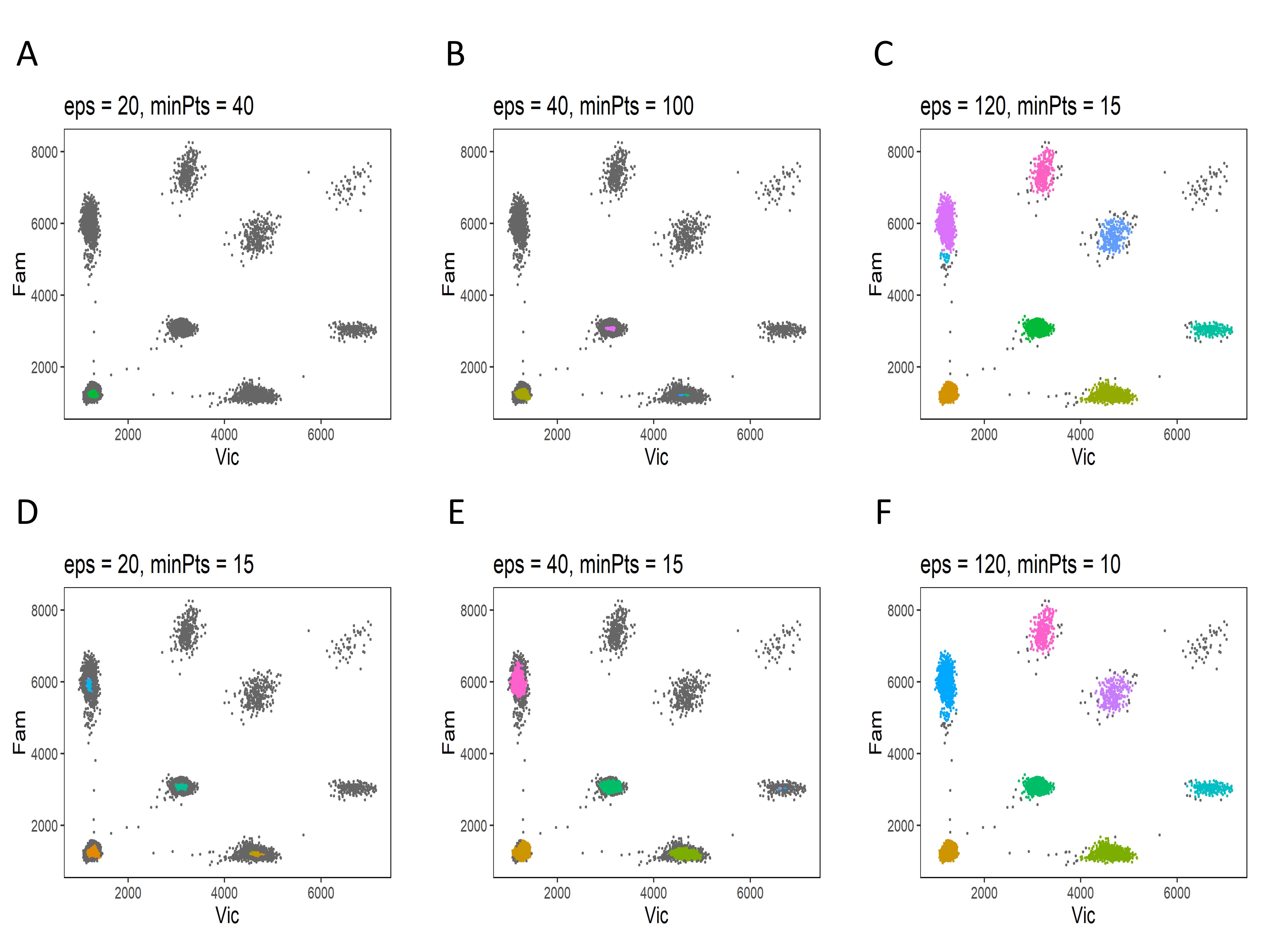
The combinations (E) and (F) identified the empty partitions cluster and all single-target clusters, therefore they are suitable for the analysis and this sample can be used as a reference.

References

Bezdek,J.C. (1981) Pattern Recognition with Fuzzy Objective Function Algorithms Springer US, Boston, MA.

Ester,M. et al. (1996) A Density-Based Algorithm for Discovering Clusters in Large Spatial Databases with Noise. In, Proceedings of the 2nd International Conference on Knowledge Discovery and Data Mining., pp. 226–231.

Hindson,B.J. et al. (2011) High-throughput droplet digital PCR system for absolute quantitation of DNA copy number. Anal. Chem., 83, 8604–8610.

Kaufman,L. and Rousseeuw,P.J. (1990) Finding Groups in Data: An Introduction to Cluster Analysis.

Lai Chung,F. and Lee,T. (1994) Fuzzy competitive learning. Neural Networks, 7, 539–551.

Mahalanobis,P.P.C. (1936) On the generalized distance in statistics. Proc. Natl. Inst. Sci. India, 2, 49–55.

Majumdar,N. et al. (2015) Digital PCR modeling for maximal sensitivity, dynamic range and measurement precision. PLoS One, 10, e0118833.

Pal,N.R. et al. (1996) Sequential competitive learning and the fuzzy c-means clustering algorithms. Neural Networks, 9, 787–796.

Rousseeuw,P.J. (1987) Silhouettes: A graphical aid to the interpretation and validation of cluster analysis. J. Comput. Appl. Math., 20, 53–65.

Whale,A.S. et al. (2016) Fundamentals of multiplexing with digital PCR. Biomol. Detect. Quantif., 10, 15–23.

Developed by Alfonso De Falco

The R package used is available on CRAN. The source code is published on Github.

Copyright 2020 Laboratoire national de santé.

Permission is hereby granted, free of charge, to any person obtaining a copy of this software and associated documentation files (the “Software”), to deal in the Software without restriction, including without limitation the rights to use, copy, modify, merge, publish, distribute, sublicense, and/or sell copies of the Software, and to permit persons to whom the Software is furnished to do so, subject to the following conditions:

The above copyright notice and this permission notice shall be included in all copies or substantial portions of the Software.

THE SOFTWARE IS PROVIDED “AS IS”, WITHOUT WARRANTY OF ANY KIND, EXPRESS OR IMPLIED, INCLUDING BUT NOT LIMITED TO THE WARRANTIES OF MERCHANTABILITY, FITNESS FOR A PARTICULAR PURPOSE AND NONINFRINGEMENT. IN NO EVENT SHALL THE AUTHORS OR COPYRIGHT HOLDERS BE LIABLE FOR ANY CLAIM, DAMAGES OR OTHER LIABILITY, WHETHER IN AN ACTION OF CONTRACT, TORT OR OTHERWISE, ARISING FROM, OUT OF OR IN CONNECTION WITH THE SOFTWARE OR THE USE OR OTHER DEALINGS IN THE SOFTWARE.